Querying 100 Million Cilium Hubble Flows on a Macbook with ClickHouse from S3Queue

ClickHouse is a powerful OLAP database designed for “analytical workloads”. Cilium is a CNCF project that does CNIs for k8s. Using the two products together allows for a powerful mix of observability and security.

Contents

• Findings
  • Running on my laptop…
  • Sample queries and speed:
  • Why is it this fast?
    • Query Schema
    • AI and ClickHouse schemas
    • ORDER BY, PARTITION BY, INDEX, and TTL
  • Optimized Queries
  • Grafana + ClickHouse + Cilium
• Setup Nextcloud + Cilium + EKS
  • Quick EKS Setup
  • Cilium Setup
  • Vector Setup
  • Nextcloud Setup

Findings

Running on my laptop…

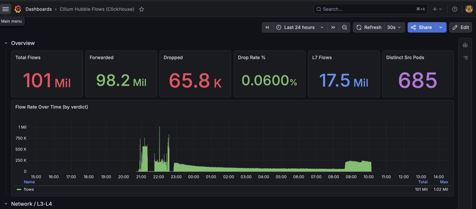
At the end of the experiment, I had almost 101 million unique flows within Cilium. I know this is a bit funny, but I ran ClickHouse on my laptop using clickhousectl and pulled the logs from an S3 bucket via S3Queue. I wanted to make a point that my Macbook Air running ClickHouse has enough power to ingest, parse, and store 100M flows from an EKS cluster that was scaled up to 250 vCPUs briefly to capture the flows from. ClickHouse is insanely powerful and is not resource hungry versus its competitors.

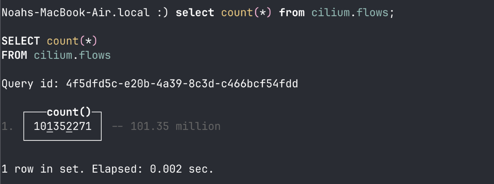
Sample queries and speed:

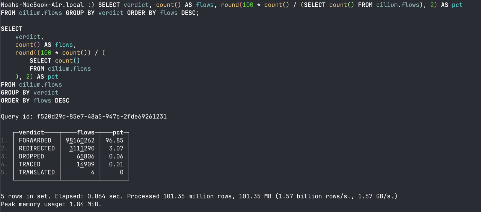
Traffic verdict, count, and overall percentage

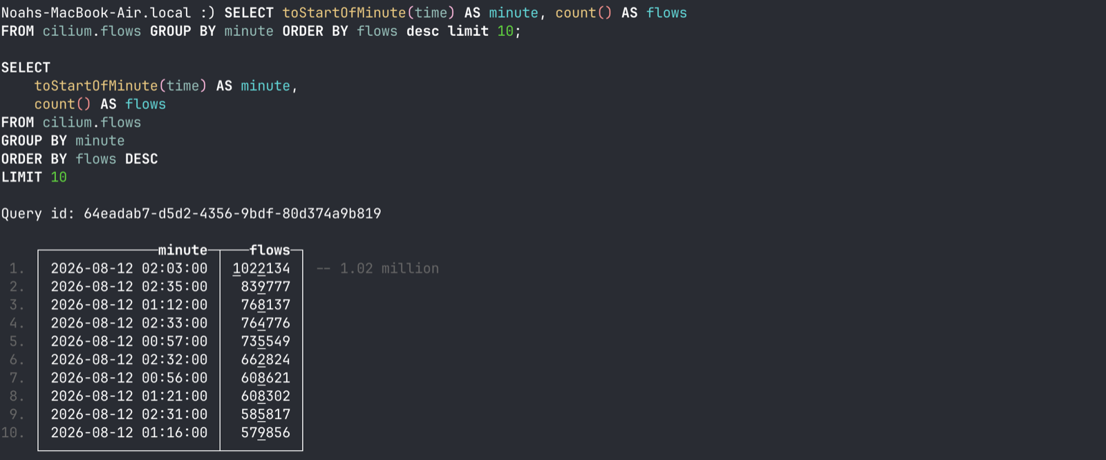
Flows per minute

Namespace to flows

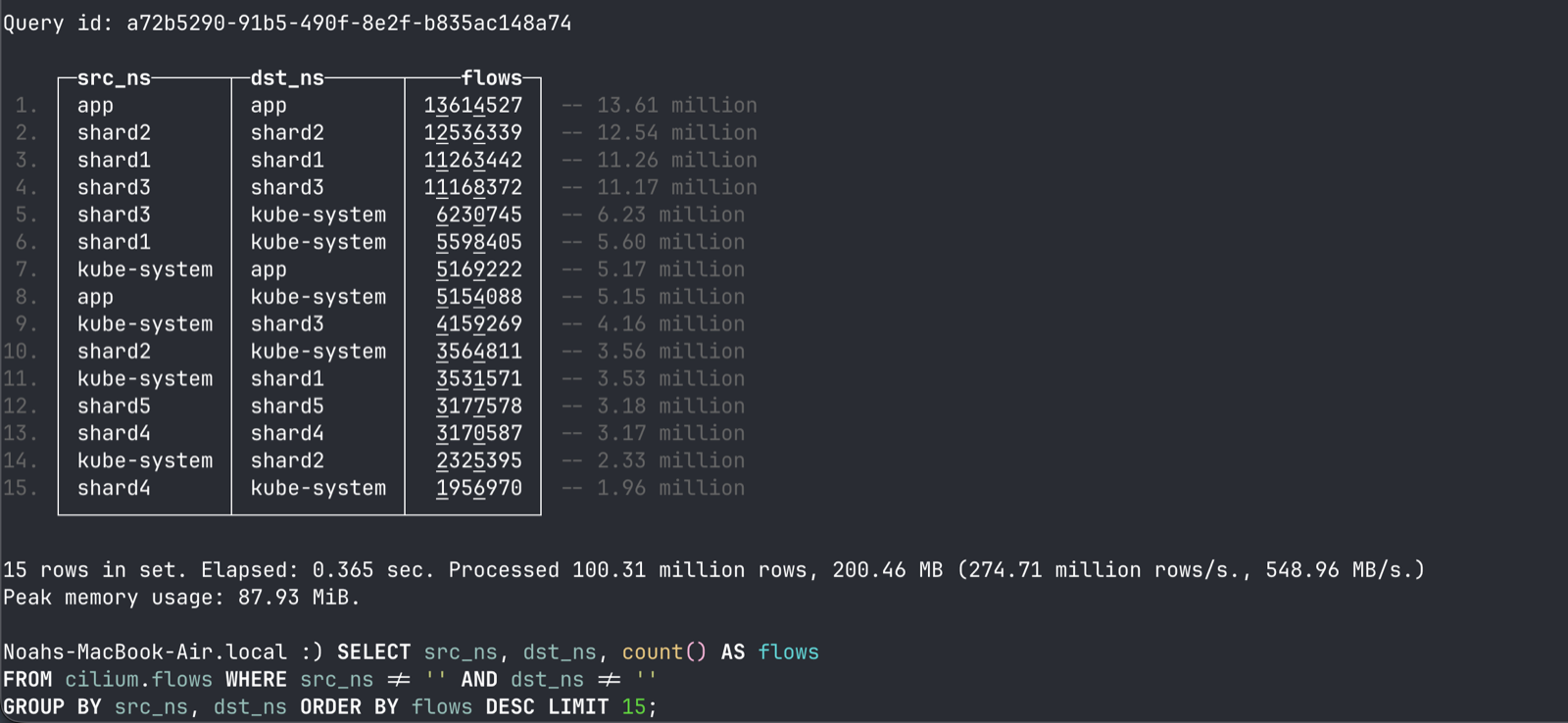
Why is it this fast?

ClickHouse is one of the fastest options here. That being said, ClickHouse was running on my laptop storing all of the data on NMVE, which is incredibly fast. Most ClickHouse instances running in the cloud will want to utilize the MergeTree engine to store the data via TTL (i.e., after one day) in S3. ClickHouse Cloud has some nifty solutions for this like using S3 One Zone. I think I’ll write another blog post about this, but I have been in scenarios using ClickHouse where the limitation was not even disk, S3, or CPU, but rather the ENI (network bandwidth/throughput) on the AWS instance type.

On top of that, ClickHouse allows very fine control over how the data is stored, which is its selling point. This allows the data querying to be done very quickly and stored very efficiently. Things like PostgreSQL, MongoDB, and Elasticsearch all abstract away most of the datatypes and how it gets stored on disk. ClickHouse embraces this design decision to bring you fast querying and enhanced columnar compression.

Query Schema

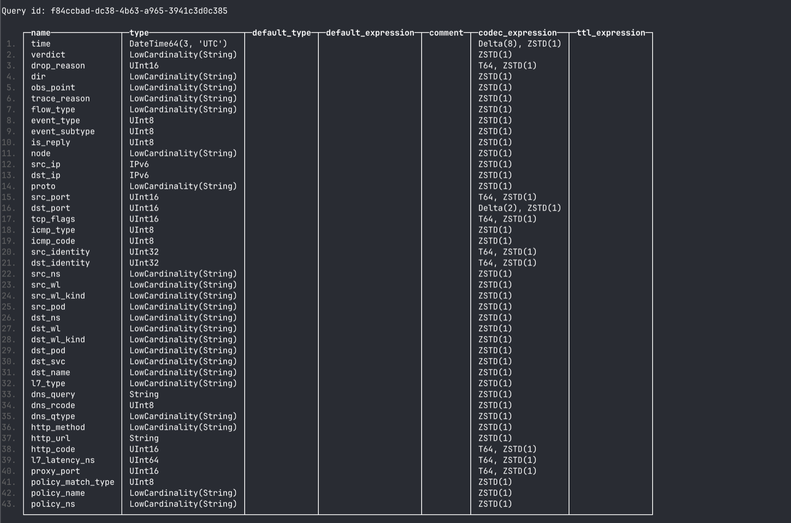
Below you can see the name, type, and codec expression being defined. Most types below are either a data primitive such as UInt8 or UInt16, and the others utilize ClickHouse’s native IPv6 datatype for storing IPs. The others are “LowCardinality” which is the sweet spot when dealing with strings within ClickHouse. Ideally, you are not storing high-cardinality string data anywhere. If you must, and make it searchable, ClickHouse recently began offering new FTS (full-text search) options when querying over text data that is more “token” based.

By using datatypes native to ClickHouse, you inherit the storage and the querying speed capabilities. Most of the work around using ClickHouse is to find a way to store your data in a way that makes sense. The returns are absurd once you align your use cases, and what data you have.

CREATE DATABASE IF NOT EXISTS cilium;

DROP TABLE IF EXISTS cilium.flows;
CREATE TABLE cilium.flows
(
    time            DateTime64(3, 'UTC') CODEC(Delta(8), ZSTD(1)),

    verdict         LowCardinality(String) CODEC(ZSTD(1)),
    drop_reason     UInt16                 CODEC(T64, ZSTD(1)),
    dir             LowCardinality(String) CODEC(ZSTD(1)),
    obs_point       LowCardinality(String) CODEC(ZSTD(1)),
    trace_reason    LowCardinality(String) CODEC(ZSTD(1)),
    flow_type       LowCardinality(String) CODEC(ZSTD(1)),
    event_type      UInt8                  CODEC(ZSTD(1)),
    event_subtype   UInt8                  CODEC(ZSTD(1)),

    is_reply        UInt8                  CODEC(ZSTD(1)),

    node            LowCardinality(String) CODEC(ZSTD(1)),

    src_ip          IPv6                   CODEC(ZSTD(1)),
    dst_ip          IPv6                   CODEC(ZSTD(1)),

    proto           LowCardinality(String) CODEC(ZSTD(1)),

    src_port        UInt16                 CODEC(T64, ZSTD(1)),

    dst_port        UInt16                 CODEC(Delta(2), ZSTD(1)),

    tcp_flags       UInt16                 CODEC(T64, ZSTD(1)),
    icmp_type       UInt8                  CODEC(ZSTD(1)),
    icmp_code       UInt8                  CODEC(ZSTD(1)),

    src_identity    UInt32                 CODEC(T64, ZSTD(1)),
    dst_identity    UInt32                 CODEC(T64, ZSTD(1)),

    src_ns          LowCardinality(String) CODEC(ZSTD(1)),
    src_wl          LowCardinality(String) CODEC(ZSTD(1)),
    src_wl_kind     LowCardinality(String) CODEC(ZSTD(1)),
    src_pod         LowCardinality(String) CODEC(ZSTD(1)),
    dst_ns          LowCardinality(String) CODEC(ZSTD(1)),
    dst_wl          LowCardinality(String) CODEC(ZSTD(1)),
    dst_wl_kind     LowCardinality(String) CODEC(ZSTD(1)),
    dst_pod         LowCardinality(String) CODEC(ZSTD(1)),
    dst_svc         LowCardinality(String) CODEC(ZSTD(1)),
    dst_name        LowCardinality(String) CODEC(ZSTD(1)),

    l7_type         LowCardinality(String) CODEC(ZSTD(1)),
    dns_query       String                 CODEC(ZSTD(1)),
    dns_rcode       UInt8                  CODEC(ZSTD(1)),
    dns_qtype       LowCardinality(String) CODEC(ZSTD(1)),
    http_method     LowCardinality(String) CODEC(ZSTD(1)),
    http_url        String                 CODEC(ZSTD(1)),
    http_code       UInt16                 CODEC(T64, ZSTD(1)),
    l7_latency_ns   UInt64                 CODEC(T64, ZSTD(1)),

    proxy_port        UInt16               CODEC(T64, ZSTD(1)),
    policy_match_type UInt8                CODEC(ZSTD(1)),
    policy_name       LowCardinality(String) CODEC(ZSTD(1)),
    policy_ns         LowCardinality(String) CODEC(ZSTD(1)),

    INDEX idx_dst_ip dst_ip TYPE bloom_filter(0.01) GRANULARITY 1,

    INDEX idx_time time TYPE minmax GRANULARITY 1
)
ENGINE = MergeTree
PARTITION BY toDate(time)
PRIMARY KEY (verdict, toStartOfHour(time), dst_ns, dst_wl)
ORDER BY  (verdict, toStartOfHour(time), dst_ns, dst_wl,
           src_ns, src_wl, dst_port, proto, time)
TTL toDateTime(time) + INTERVAL 14 DAY DELETE
SETTINGS
    ratio_of_defaults_for_sparse_serialization = 0.9,
    min_age_to_force_merge_seconds = 3600,
    min_age_to_force_merge_on_partition_only = 1,
    ttl_only_drop_parts = 1;

AI and ClickHouse schemas

Okay so if you are new to ClickHouse, ask Claude Code or Codex to look at the data you are using, and then write a ClickHouse schema for it. More often than not, it will write a pretty good schema. However, in my experience, AI will not think through all of the scaling possibilities and choose the MOST optimal way to store and hence query data. I used AI to generate my schema, and then made some directory style edits to how I wanted it to go. For instance AI is very gung-ho on storing IPv4 and IPv6 separately, which is stupid, because ClickHouse’s IPv6 data type supports storing and querying IPv4 addresses. So be careful in evaluating all the decisions it has made.

ORDER BY, PARTITION BY, INDEX, and TTL

These are the most important things to get right when working with ClickHouse. These define where and how long the data lives, how ClickHouse chooses to store the data to query over it, and any additional searching mechanisms like INDEX that you choose.

IP searching is a bit interesting within ClickHouse. There are very few cases where I can think of that you would want to make your ORDER BY statement include an IP column. It is totally possible, but when choosing things to order by, you want to generally order by columns that are low-cardinality, and while IPv4 (for example) is a fixed range, it is well past the ability to be treated as a low-cardinality dataset. Using bloom filters for IPs, and then using order by statements wrapped around timed events, often work the best. However, if almost all of your queries are searching by one high-cardinality datatype, then it is not a hard limit and you can order by them.

In this case, where the bloom filter is applied, ClickHouse can more optimally skip to search over granules that most likely do not contain the information.

“PARTITION BY” is another piece to this puzzle. This allows you to create parts that physically group together the data. By telling ClickHouse in our example that we want to partition it by the toDate(time), we are telling it that all of the data for one day should live together.

You could partition by something more granular, but that does not automatically make something like a time-series query faster. Using partitions should be for a data management tool or lifecycle segmentation. ClickHouse has better tools for pruning mechanisms when searching across data. By making the data parts you are searching over too fine, you lose speed by just searching over them vs the data inside them (especially bad for object storage). The idea here is to keep it relatively coarse.

So if you have 14 days’ worth of data, and your data was located on the 3rd day, and you partition it by day, ClickHouse could skip over all the per-day partitions that would not have the data you were looking for and JUST search the 3rd day.

“ORDER BY” is the next most important decision you can make when building a table/db within ClickHouse. In our schema we have verdict, toStartOfHour(time), dst_ns, dst_wl, src_ns, src_wl, dst_port, proto, time. This means that when a Cilium log first arrives, it gets sent to the correct partition (logically should be the most recent unless you have some crazy delay), and then it gets stored by the ordering of the values here. In our case, we are interested in knowing for most queries what the verdict was. This demo had 5 verdicts:

┌─verdict────┬────flows─┬───pct─┐
1. │ FORWARDED  │ 98160262 │ 96.85 │
2. │ REDIRECTED │  3111290 │  3.07 │
3. │ DROPPED    │    65806 │  0.06 │
4. │ TRACED     │    14909 │  0.01 │
5. │ TRANSLATED │        4 │     0 │
   └────────────┴──────────┴───────┘
   5 rows in set. Elapsed: 0.066 sec. Processed 101.35 million rows, 101.35 MB (1.55 billion rows/s., 1.55 GB/s.)

So log comes in, sorts into correct day, sorts into verdict, and then sorts by the other variables. This makes selective queries against a specific verdict extremely cheap.

After that come the time, namespaces, workload, dst port, type, and then exact time. The toStartOfHour makes sense for dashboarding later on, since most dashboards would care about the hour range.

If I’m a security engineer, or a DevOps engineer, and I want to know what the top verdict per namespace is, or the inverse of that being top namespace with x verdict, that makes investigations like these very straightforward. Drilling down after each step, you lose some optimizations, but after a certain while with only 40-something columns of data that is partitioned and stored correctly, ClickHouse is going to make up for it in speed.

Here is an example of this working: if I want to grab just the count of verdict “x” happening, it only scans 8.15K-ish rows, rather than every log to count up the verdict happening. This is a crude example, because it really is using the PRIMARY KEY…more below.

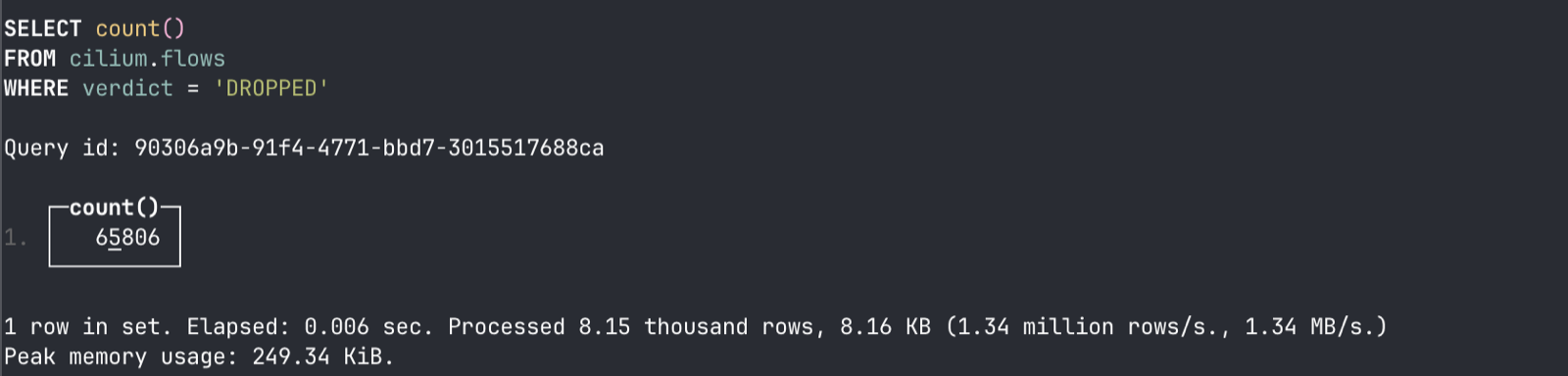
“PRIMARY KEY” is the next sister element to the partition system. This is a sparse index that ClickHouse will keep per data part within MergeTree. In our case we had PRIMARY KEY (verdict, toStartOfHour(time), dst_ns, dst_wl). You want to keep the primary key statement with fewer elements than the ORDER BY key statement, as the goal here is to build a primary index per the first order by elements, otherwise the sparse index gets larger and outgrows its usefulness when pruning granules. Running an EXPLAIN statement helps clear up what is happening with our verdict query from above:

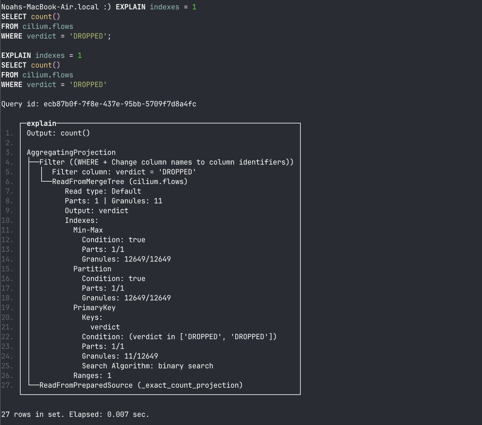
Since we were not searching by time, the min-max filter did not help us. The partition did not really help us either, as most of the data is just on one partition since the demo environment did not get run long. The next step with the primary key gathers the major performance gains. It whittles it down from 12649 granules (in this case, and with any default ClickHouse schema, the default is 8192 rows per granule) to 11 via binary search. Those 11 granules are what ClickHouse would need to scan to read the matching flows off disk, but the _exact_count_projection in the EXPLAIN output shows it actually short-circuits that read entirely and returns the exact count (65,806) straight from the index, which is why the query only processed 8.15 thousand rows of index metadata instead of scanning the granules themselves.

“INDEX name expr TYPE”: these are the skip indexes used within the schema. You can think of them like secondary pruning mechanisms within ClickHouse. Unlike PostgreSQL and its use of B-tree indexes, ClickHouse’s skip indexes instead examine chunks of data to determine whether the data resides there. Here is an example for querying by IP address:

SELECT count()
FROM cilium.flows
WHERE dst_ip = toIPv6('::ffff:3.146.14.246');

Automatically this is not going to get any of the ordering by benefits we talked about above. It does not care about the verdict, time, or any of the other high-level keys. It is searching all the logs for an IPv4 address cast to an IPv6 store.

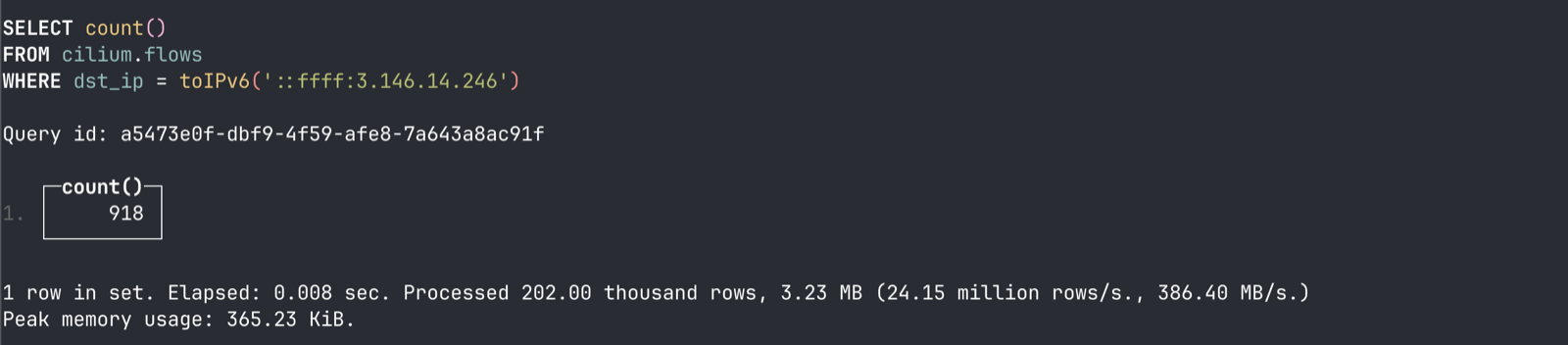
That being said, the query only scans 202K rows out of 100M rows and returns insanely fast. How is it doing this?

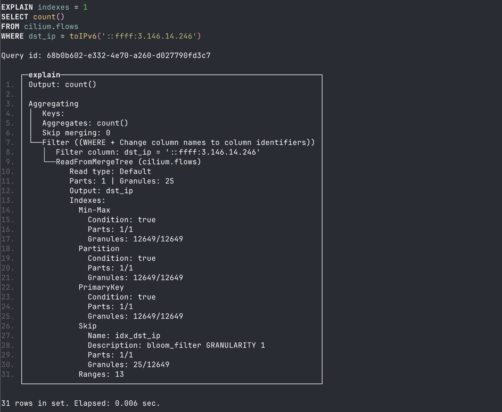
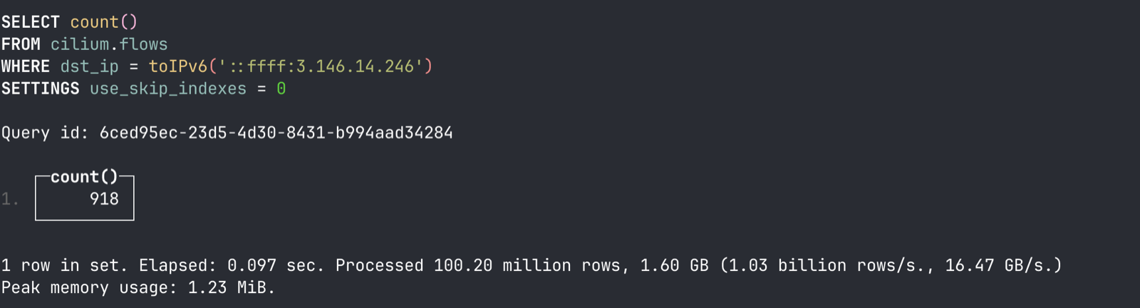
If you append an EXPLAIN statement pre-query, you get a nice visualization of how the query logic works. From a total of 12.6K granules, it finds 25 of them that might contain the data it is looking for, scans those, and returns the count of 918. Running this query again with SETTINGS use_skip_indexes = 0 forces ClickHouse to scan through every row in the table to find the count of that IP. Another thing to note is that bloom filters are designed to be accurate but at a loss of the amount of data they need to scan over in the scenario. So it scaned 25 granules, but the data is in fewer than that. Far better than scanning all 12.6K granules whilest providing confidence that the value you get is the accurate value.

Optimized Queries

Below are some screenshots of queries that are optimized to not scan the entire 100M logs while still deriving absolute results.

Querying for namespace verdicts:

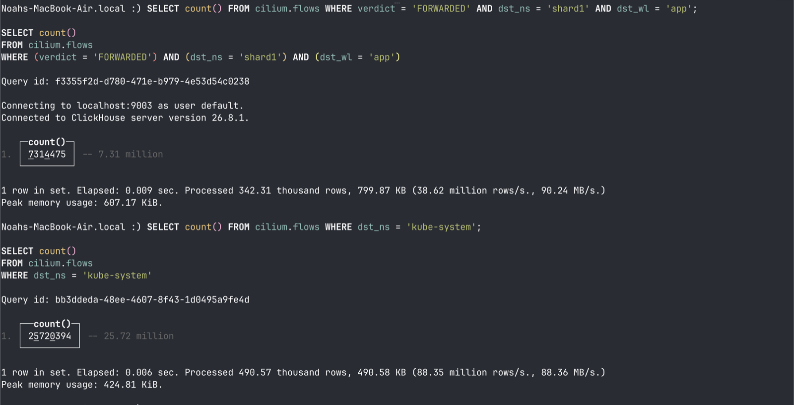
Querying for dropped traffic to a certain namespace/workload and querying port/protocol that is problematic:

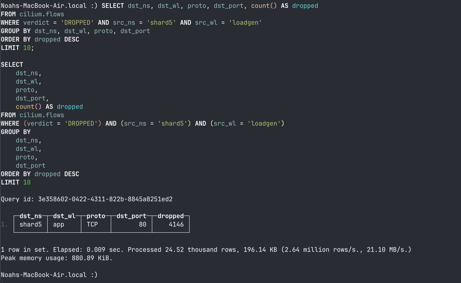
Then taking it a step further and querying the pod that the traffic was dropped coming from:

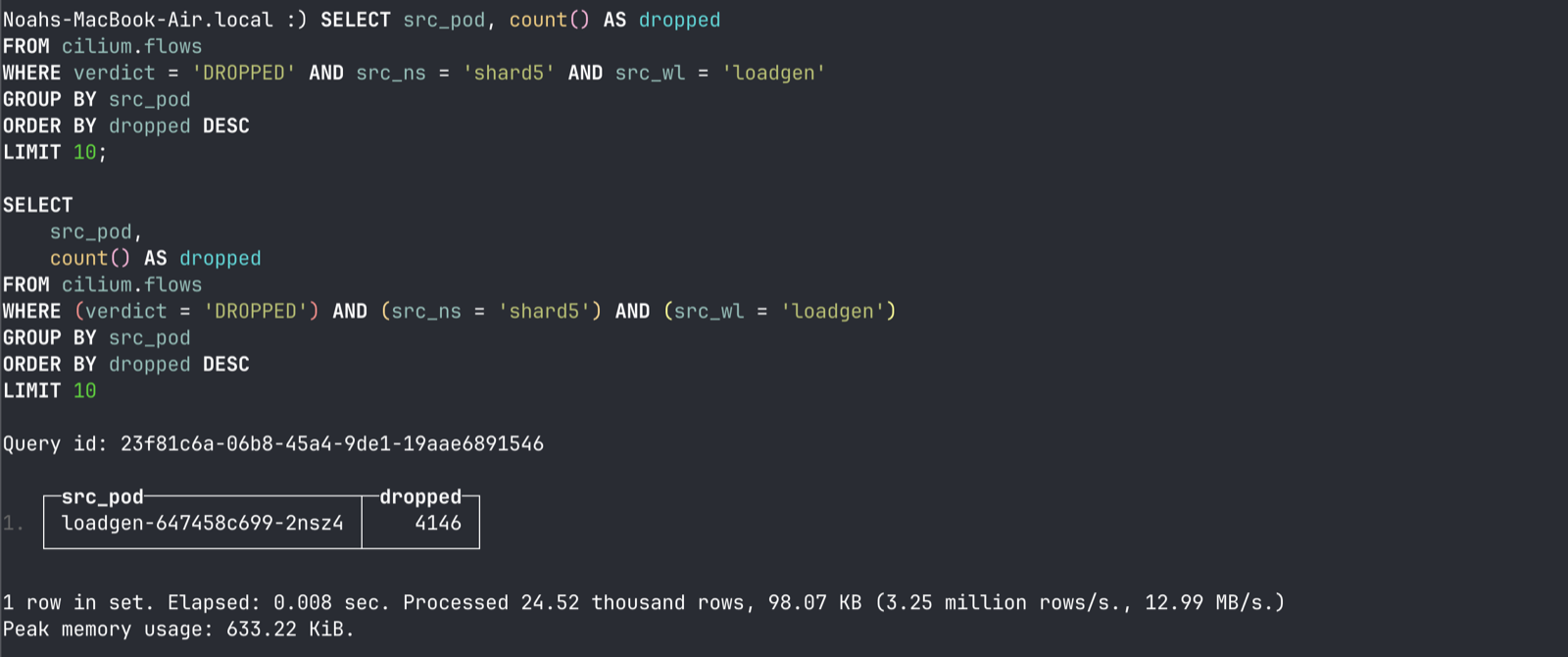
These queries are designed specifically to use the schema design that we created for this env.

Grafana + ClickHouse + Cilium

What good is a log database if you can not query it? Grafana has some beautiful dashboard tools and AI MCPs that allow you to quickly create dashboards that use these blazing-fast ClickHouse databases.

Some cool screenshots (created via Claude Code and Grafana MCP)

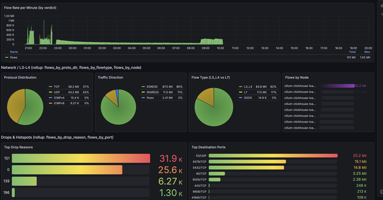
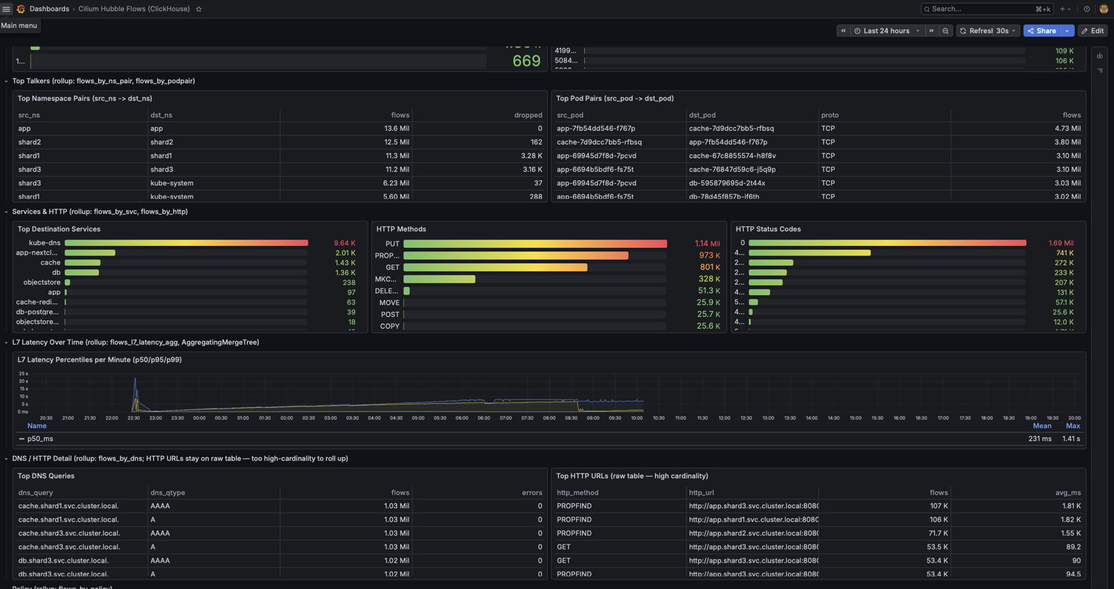
Grafana dashboards present a unique opportunity within ClickHouse. Dashboards are mostly interested in aggregate data, not specifics. Even specific counts can be aggregate data within a certain time frame. I went ahead and created a few additional tables within ClickHouse to support these dashboards that use the SummingMergeTree engine.

The reasoning behind this decision is that you do not want every dashboard refresh to be scanning through every log line even though ClickHouse can do this quickly. You will quickly rack up a costly S3 bill. Because we are using S3Queues, ClickHouse requires an MV table before a destination table. This is also good because we can send the data to multiple destination tables at once from one S3Queue. Ideally most panels within your dashboard will query a respective “roll-up table”. ClickHouse has the idea of SummingMergeTree just for this reason; it stores a “counter” per se depending on the data you tell it to track.

Here is an example:

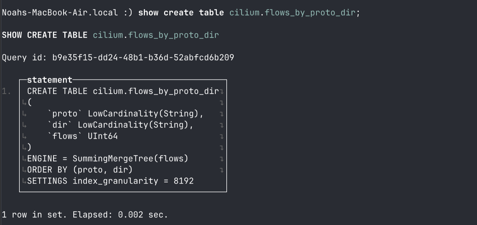
This table effectively allows ClickHouse to treat incoming data with this evaluation:

When rows with the same sorting key are merged, sum the flows column.

This is not a great example as this SummingMergeTree is not time-bound. Most of the time you want your panels to be time aware and respond well to time-based queries from within Grafana.

Setup Nextcloud + Cilium + EKS

To generate 100M logs from Cilium to put into ClickHouse, I am spinning up an EKS cluster with multiple Nextcloud (an open-source filesystem Dropbox-like alternative) deployments and hitting their HTTP endpoints simulating users (file read, file upload, file delete, directory read, etc). Nextcloud was set up to use PostgreSQL, Redis, MinIO, etc as dependencies to generate as much in-cluster traffic as possible.

Quick EKS Setup

I did a quick EKS setup with eksctl, and grew the node pool as needed. I set this up without the AWS VPC CNI, detailed further in the Cilium section below.

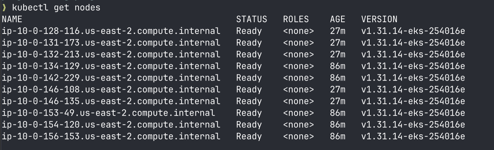
It grew to 254 vCPUs at one point when I was trying to scale the Nextcloud deployments (my poor AWS account)!

kubectl get nodes -o json | jq -r '[.items[].status.allocatable.cpu | if endswith("m") then rtrimstr("m") | tonumber / 1000 else tonumber end] | add | "\(.) cores"'
254.2399999999999 cores

Cilium Setup

Cilium was the primary CNI, and the EKS cluster was configured to not use the default AWS VPC CNI from the start. All traffic from any node would be captured by Cilium, in large part by its use of eBPF along with nftables/iptables.

cilium install \
  --set ipam.mode=cluster-pool \
  --set ipam.operator.clusterPoolIPv4PodCIDRList='{10.244.0.0/16}' \
  --set routingMode=tunnel \
  --set tunnelProtocol=vxlan \
  --set kubeProxyReplacement=true \
  --set k8sServiceHost=auto \
  --set hubble.enabled=true \
  --set hubble.relay.enabled=true \
  --set 'hubble.export.static.enabled=true' \
  --set 'hubble.export.static.filePath=/var/run/cilium/hubble/events.log'

This was the install command. The Hubble config at the bottom told each DaemonSet on every node to dump the logs to events.log, which we would pick up with Vector as a DaemonSet as well.

Vector Setup

Vector pods running below, one for each node:

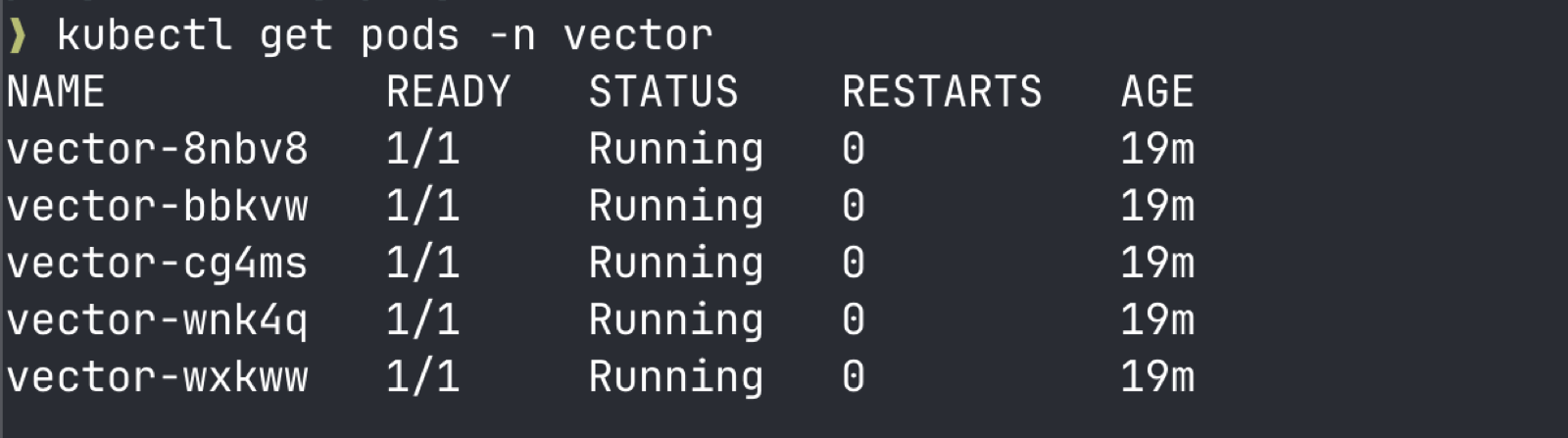
Here is my Vector config for reference (inside the ConfigMap for Vector):

  vector.toml: |
    [sources.hubble_flows]
    type = "file"
    include = ["/var/run/cilium/hubble/events.log*"]

    [sinks.s3]
    type = "aws_s3"
    inputs = ["hubble_flows"]
    bucket = "hubble-flow-logs-demo-x7k2p9"
    region = "us-east-2"
    key_prefix = "hubble-flows/dt=%Y-%m-%d/%H/${NODE_NAME}-"
    compression = "gzip"
    encoding.codec = "json"
    framing.method = "newline_delimited"
    batch.max_bytes = 10485760
    batch.timeout_secs = 30

The important takeaways here are that the output to S3 is configured to compress the logs before sending them to S3 with gzip, the logs are compressed plus arranged in NDJSON style with one JSON line per newline, and that there are buffering limits to both size and time. Whichever criteria becomes true first, Vector will ship them out. Some other components of the Vector setup included ensuring there was an IRSA role that it could assume that had correct S3 permissions against the bucket, and what ConfigMap the Vector config lived in.

Nextcloud Setup

This was probably the worst Nextcloud deployment in history, lol, but it got the job done. Simple PHP container and then wired up to all the other moving parts.

kubectl get deployment app-nextcloud -o yaml -n app
apiVersion: apps/v1
kind: Deployment
metadata:
  annotations:
    deployment.kubernetes.io/revision: "3"
    meta.helm.sh/release-name: app
    meta.helm.sh/release-namespace: app
  creationTimestamp: "2026-08-12T00:46:50Z"
  generation: 3
  labels:
    app.kubernetes.io/component: app
    app.kubernetes.io/instance: app
    app.kubernetes.io/managed-by: Helm
    app.kubernetes.io/name: nextcloud
    app.kubernetes.io/version: 34.0.2
    helm.sh/chart: nextcloud-9.2.5
  name: app-nextcloud
  namespace: app
  resourceVersion: "14869"
  uid: 25d3ee7d-e02e-442e-872c-4b76da1fb492
spec:
  progressDeadlineSeconds: 600
  replicas: 1
  revisionHistoryLimit: 10
  selector:
    matchLabels:
      app.kubernetes.io/component: app
      app.kubernetes.io/instance: app
      app.kubernetes.io/name: nextcloud
  strategy:
    type: Recreate
  template:
    metadata:
      annotations:
        hooks-hash: 44136fa355b3678a1146ad16f7e8649e94fb4fc21fe77e8310c060f61caaff8a
        nextcloud-config-hash: 2c620d6eac4314c9a69fdfb299af32077aa552fd06db46dbb6c56d93803f75f6
        php-config-hash: 44136fa355b3678a1146ad16f7e8649e94fb4fc21fe77e8310c060f61caaff8a
      creationTimestamp: null
      labels:
        app.kubernetes.io/component: app
        app.kubernetes.io/instance: app
        app.kubernetes.io/name: nextcloud
    spec:
      containers:
      - env:
        - name: POSTGRES_HOST
          value: db-postgresql
        - name: POSTGRES_DB
          value: app
        - name: POSTGRES_USER
          valueFrom:
            secretKeyRef:
              key: db-username
              name: app-db
        - name: POSTGRES_PASSWORD
          valueFrom:
            secretKeyRef:
              key: db-password
              name: app-db
        - name: DATABASE_URL
          value: postgres://$(POSTGRES_USER):$(POSTGRES_PASSWORD)@$(POSTGRES_HOST)/$(POSTGRES_DB)
        - name: REDIS_HOST
          value: cache-redis-master
        - name: REDIS_HOST_PORT
          value: "6379"
        - name: REDIS_URL
          value: redis://:$(REDIS_HOST_PASSWORD)@$(REDIS_HOST):$(REDIS_HOST_PORT)
        - name: NEXTCLOUD_ADMIN_USER
          valueFrom:
            secretKeyRef:
              key: nextcloud-username
              name: app-nextcloud
        - name: NEXTCLOUD_ADMIN_PASSWORD
          valueFrom:
            secretKeyRef:
              key: nextcloud-password
              name: app-nextcloud
        - name: NEXTCLOUD_TRUSTED_DOMAINS
          value: '*'
        - name: OPENMETRICS_ALLOWED_CLIENTS
          value: 127.0.0.1,10.42.0.0/16,10.43.0.0/16
        - name: NEXTCLOUD_DATA_DIR
          value: /var/www/html/data
        - name: OBJECTSTORE_S3_SSL
          value: "false"
        - name: OBJECTSTORE_S3_USEPATH_STYLE
          value: "true"
        - name: OBJECTSTORE_S3_AUTOCREATE
          value: "true"
        - name: OBJECTSTORE_S3_REGION
          value: us-east-1
        - name: OBJECTSTORE_S3_PORT
          value: "9000"
        - name: OBJECTSTORE_S3_STORAGE_CLASS
          value: STANDARD
        - name: OBJECTSTORE_S3_HOST
          value: objectstore-minio
        - name: OBJECTSTORE_S3_BUCKET
          value: app-data
        - name: OBJECTSTORE_S3_KEY
          value: minioadmin
        - name: OBJECTSTORE_S3_SECRET
          value: minioadmin
        - name: OBJECTSTORE_S3_SSE_C_KEY
        - name: OVERWRITEPROTOCOL
          value: http
        image: docker.io/library/nextcloud:34.0.2-apache
        imagePullPolicy: IfNotPresent
        name: nextcloud
        ports:
        - containerPort: 80
          name: http
          protocol: TCP
        resources:
          limits:
            cpu: "12"
            memory: 48Gi
          requests:
            cpu: "6"
            memory: 16Gi
        terminationMessagePath: /dev/termination-log
        terminationMessagePolicy: File
        volumeMounts:
        - mountPath: /var/www/
          name: nextcloud-main
          subPath: root
        - mountPath: /var/www/html
          name: nextcloud-main
          subPath: html
        - mountPath: /var/www/html/data
          name: nextcloud-main
          subPath: data
        - mountPath: /var/www/html/config
          name: nextcloud-main
          subPath: config
        - mountPath: /var/www/html/custom_apps
          name: nextcloud-main
          subPath: custom_apps
        - mountPath: /var/www/tmp
          name: nextcloud-main
          subPath: tmp
        - mountPath: /var/www/html/themes
          name: nextcloud-main
          subPath: themes
      dnsConfig: {}
      dnsPolicy: ClusterFirst
      restartPolicy: Always
      schedulerName: default-scheduler
      securityContext:
        fsGroup: 33
      terminationGracePeriodSeconds: 30
      volumes:
      - name: nextcloud-main
        persistentVolumeClaim:
          claimName: app-nextcloud-nextcloud

❯ kubectl get svc -n app
NAME                   TYPE        CLUSTER-IP       EXTERNAL-IP   PORT(S)             AGE
app-nextcloud          ClusterIP   172.20.123.9     <none>        8080/TCP            47m
cache-redis-headless   ClusterIP   None             <none>        6379/TCP            49m
cache-redis-master     ClusterIP   172.20.225.163   <none>        6379/TCP            49m
db-postgresql          ClusterIP   172.20.11.55     <none>        5432/TCP            49m
db-postgresql-hl       ClusterIP   None             <none>        5432/TCP            49m
objectstore-minio      ClusterIP   172.20.49.166    <none>        9000/TCP,9090/TCP   48m

All of this together created the setup needed for my Cilium experiment! Thank you for reading!